Developer Guides
zkSNARKs and PLONK
Overview
zkSNARKs are powerful modern cryptography primitives used to prove the correct execution of an arbitrary computation without the need for a verifier to re-execute that computation. In addition to that, zkSNARKs have the ability to reveal only some parts of the computation and retain the rest as a secret, all while proving correctness of 100% of it.
Common use cases for zkSNARKs in modern blockchains are:
- proving the correct execution of a smartcontract endpoint without requiring all validators in the network to re-execute the corresponding transaction,
- implementing privacy-preserving protocols such as anonymous voting and payments.
The acronym "zkSNARK" stands for Zero-Knowledge Succinct Non-interactive Argument of Knowledge:
- zero-knowledge means the proven computation is not revealed, except for the parts the prover chooses to reveal;
- succinct means the size of the proof is sublinear in the size of the original computation (in fact, the zkSNARK scheme used in Libernet results in constant-size proofs of about 1 KiB each);
- non-interactive means the verification protocol does not require a challenge-response roundtrip;
- argument of knowledge indicates that the prover really had the full trace of the computation, notwithstanding the above requirements.
Libernet uses zkSNARKs in a few different contexts, for example anonymous payments towards incognito accounts. Our zkSNARK protocol is based on KZG polynomial commitments over the BLS12-381 elliptic curve, and PLONK arithmetization. It uses the Poseidon algebraic hash for hashing.
This page describes the full PLONK protocol that we use in Libernet in detail, but it assumes knowledge of KZG. Be sure to understand everything in Dankrad Feist's article before moving on.
Circuits
In the zkSNARK world a computation is conceptually rendered as a circuit with gates and wires. The gates represent basic arithmetic operations such as addition and multiplication, and the wires connect the inputs and outputs of the gates.
As an example, consider the following circuit:
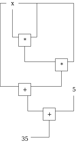
It's easy to see how this encodes the computation of . A prover with this circuit can produce a zkSNARK proof that convinces a verifier of a statement like "I have a secret number such that ", without revealing . This is a simple example so it's easy to find out that the number would be , but zkSNARKs enable complex protocols such as anonymous voting and payments where some elements of the computation remain secret.
Evaluation Domain and Polynomial Interpolation
Libernet uses the BLS12-381 elliptic curve, so all of its zkSNARK circuits are evaluated on the scalar field of that curve. The field has the following ~256 bit order:
r = 0x73eda753299d7d483339d80809a1d80553bda402fffe5bfeffffffff00000001So the values carried by the wires of our circuits are ~256 bit integers.
In zkSNARKs we encode all computation in polynomials. To see how a polynomial can encode an ordered list of integers, consider the following list of pairs:
(0, 33)
(1, 10)
(2, 24)
(3, 49)
To encode the ordered list of integers [33, 10, 24, 49] we can use a polynomial that crosses the
points represented by the above pairs. This is achieved by polynomial interpolation, and the
resulting polynomial would evaluate to 33 in 0, to 10 in 1, etc., effectively encoding the
original list at the coordinates 0, 1, 2, and 3.
There are two distinct approaches to implementing polynomial interpolation: Lagrange interpolation and the Fast Fourier Transform. Algorithms based on Lagrange interpolation take time where is the number of points to interpolate, so in Libernet we use the Fast Fourier Transform which takes time. However, some parts of our PLONK protocol also use Lagrange basis polynomials for other purposes (more on that later).
The Fast Fourier Transform algorithm is significantly faster than Lagrange interpolation but has two important restrictions:
- the number of interpolated points must be a power of 2,
- and the X coordinates of the points cannot have arbitrary values, they must be powers of an N-th root of unity.
As a quick refresher, an -th root of unity is a number such that . The FFT algorithm requires the X-coordinates of the interpolated points to be:
where is a power of 2.
When working with standard math tools the equation has exactly complex solutions. For example, for the four solutions are , , , and (with being the imaginary unit ).
In modular arithmetic things work differently, but since the BL12-381 scalar field has prime order, Fermat's Little Theorem shows us that the equation can still be satisfied. In fact, the field has the following well-known -th root of unity:
0x16a2a19edfe81f20d09b681922c813b4b63683508c2280b93829971f439f0d2bThere are different powers of this number, allowing us to interpolate at most (or 4,294,967,296) points using the Fast Fourier Transform. From there we can adapt the FFT algorithm to run on any number of points that's a power of two less than or equal to .
Let's define:
We can obtain a -th root of unity from the -th root of unity as follows:
In fact:
Given all the above, we'll often work with powers of rather than plain naturals as our evaluation domain. Instead of encoding the following points:
(0, 33)
(1, 10)
(2, 24)
(3, 49)
we'll use the FFT algorithm to encode the following points:
(w0^0, 33)
(w0^1, 10)
(w0^2, 24)
(w0^3, 49)
where w0 is a -th root of unity , in this case .
Note
In the following we will use instead of for notational simplicity. We still use to indicate the (padded) size of the circuit, so you'll often see things like .
The Fast Fourier Transform and other algorithms on polynomials are implemented in the poly module
of our crypto library.
Witnesses and Constraints
Proving the correct execution of an arbitrary computation takes the following steps:
- both the prover and the verifier become aware of the same circuit (gates and wires);
- the prover runs the computation, providing input values to the circuit, computing all intermediate values, and obtaining the output values;
- the prover provides:
- a proof of knowledge of the above values;
- a proof that the above values satisfy certain constraints;
- the verifier verifies the above proofs without any challenge-response roundtrip, just checking them against the original circuit.
The set of values produced at step #2 is known as the witness. You can think of it as the "execution trace" of the computation, since it includes all intermediate values. In the PLONK proving scheme the witness is organized in three columns of equal height:
- the column of the left-hand side inputs of all gates,
- the column of the right-hand side inputs of all gates,
- and the column of the outputs of all gates.
The i-th row of each column contains the corresponding value for the i-th gate.
For example, the circuit above would have the following witness when the secret input is set to 3:
| LHS | RHS | Out |
|---|---|---|
| 3 | 3 | 9 |
| 9 | 3 | 27 |
| 3 | 27 | 30 |
| 30 | 5 | 35 |
Proving knowledge of the witness (as per point 3a above) is easy:
- the columns of the witness are padded with zeros until their size is a power of 2,
- each column is then encoded as a polynomial using the FFT algorithm,
- the polynomial is committed to G1 as per KZG and the 3 commitments are provided as proof,
- KZG openings are provided to reveal the public parts of the computation.
However, this doesn't prove that the witnessed values really did result from computing the known circuit. To achieve that we need to enforce a set of polynomial equations that characterize the circuit. These equations are known as constraints. The initial definition of a circuit, which is performed only once and ahead of time, results in two types of constraints: gate constraints and wire constraints, discussed below. The prover and the verifier can perform this initial definition process independently, but it must results in exactly the same constraints for the proofs to be valid.
Gate Constraints
In the PLONK proving scheme each gate defines a polynomial constraint of the following form:
where:
- is the left-hand side input of the gate,
- is the right-hand side input of the gate,
- is the output of the gate,
- the factors are constants specific to the gate.
For example, an addition gate would have:
effectively yielding the constraint:
A multiplication gate would instead have:
resulting in:
Note
Negative values don't exist in our scalar field. What we actually do for the above gate types to achieve the same result is to set , to which -1 is congruent. is the prime order of the BLS12-381 scalar field, provided above.
Defining a circuit with gates would result in values for , values for , and so on, meaning we can encode the five columns in five corresponding polynomials . Let , , and be the polynomials encoding the three witness columns. After interpolating all polynomials we have:
Note that the can (and in fact must) be interpolated ahead of time, so they only contribute to the cost of the setup phase (in both the prover and the verifier) but not to the proving or verification cost.
This equation is a single polynomial equation that we can commit to and for which we can provide KZG openings on one or more challenge points. To maintain the protocol non-interactive we can use the Fiat-Shamir heuristic to determine the challenge points, e.g. we can compute them by hashing the polynomial commitments of the witness columns.
To prove that the witness really was computed by the circuit gates defined by we need to prove:
for all , meaning that our constraint equation must be zero on all points of the evaluation domain , , , ..., . In other words, all powers of must be roots of the polynomial . That means can be rewritten as:
where is a quotient polynomial resulting from the division of by .
The divisor is a polynomial that vanishes on all the evaluation domain and doesn't have any other roots. It's sometimes known as the zero polynomial, and we'll indicate it with .
We also use the following notation:
meaning that the polynomial division of by yields a zero remainder.
Determining the coefficients of is very straightforward because the condition of vanishing on all -th roots of unity is simply defined by the equation:
so we have:
Circling back to the problem of proving that is satisfied, i.e. zero on all powers of , we can adopt the following protocol:
- the prover determines a challenge value using the Fiat-Shamir heuristic;
- the prover generates the coefficients of by multiplying the polynomials by the witness polynomials as per the definition of ;
- the prover divides by using polynomial long division and obtains (if really is satisfied there must be no remainder);
- the prover commits to and opens it at .
Note that the existence of without any remainder implies that is divisible by and is therefore zero on all the domain and fully satisfied. Thanks to that, on the verifier side we just need to verify the KZG openings for , , , and and check:
This is however not yet enough to prove that the witness really fits the circuit: our protocol so far checks that each gate has worked correctly but doesn't check that the gates were connected as intended. To achieve the latter we need to check wire constraints.
Wire Constraints
This is the most complex part of PLONK.
Proving that the gates of the circuit are connected as intended boils down to proving that specific groups of cells of the witness table have equal values, without revealing the whole witness.
Here is once again the full witness table of our sample circuit:
| LHS | RHS | Out |
|---|---|---|
| 3 | 3 | 9 |
| 9 | 3 | 27 |
| 3 | 27 | 30 |
| 30 | 5 | 35 |
Based on the wiring of the circuit, we need to partition the wires as follows and prove that each partition contains identical values. We use , , and to indicate the -th row of the left input, right input, and output column, respectively.
- (value 3)
- (value 9)
- (value 27)
- (value 30)
- (value 5)
- (value 35)
The core insight is that the witness wouldn't change if we permuted the elements of each partition arbitrarily, because they have identical values. Therefore, to achieve our goal we'll build a polynomial expression based on permutations of the X coordinates of our domain, .
Let's first analyze a simplified case that works on a single witness column polynomial . Let be a permutation of the evaluation domain that rotates or otherwise rearranges the coordinates of each wire partition, and let be the -th element of the permutation. Let and be two challenge values computed with Fiat-Shamir (not the same as the challenge used for gate constraints). We define the coordinate pair accumulator of as follows:
This gives us an intuition of how partition-wise wire equality is proven: since the coordinates in the denominator are permuted, the value of the coordinate pair accumulator is 1 iff the factors in the denominator remain equal to those in the numerator except for their order -- in other words, iff the permutation didn't change anything in the overall expression. So proving that all wire constraints are satisfied reduces to proving that the coordinate pair accumulator product equals 1 for that witness.
Let's now extend this technique to work with three different witness columns , , and . We will build a "unified" coordinate pair accumulator multiplying the individual accumulators of the three columns together, but to avoid collisions among the X coordinates we need to introduce two constants and in the accumulators of and respectively (we can use 1 as the constant for ) and we need to change the construction of accordingly. In Libernet we set and .
Specifically, we will now construct three separate permutations , , and . To do that, we first lay out the X coordinates of , , and in a single array with length (note that the coordinates of and are multiplied by and respectively, so all values are different):
Then we rotate or otherwise rearrange the elements of each partition. It's okay to use a predefined permutation algorithm, e.g. rotation by a fixed offset; the only requirement is that each partition has a permutation with exactly 1 cycle. For example, if we used a rotation by 1 slot of our sample circuit above we'd get the following permutation:

resulting in:
Once we have this permuted, -long sequence, we get:
- by taking the first elements,
- by taking the next elements,
- by taking the last elements.
In our example we'd get:
These three sequences can be encoded in three polynomials, each mapping an element of the evaluation domain to the corresponding permuted element. Following our example, the polynomial is obtained by interpolating the following points:
(w^0, w^2)
(w^1, k2 * w^0)
(w^2, k1 * w^1)
(w^3, k2 * w^2)
For we have:
(w^0, w^0)
(w^1, k1 * w^0)
(w^2, k2 * w^1)
(w^3, k1 * w^3)
And for :
(w^0, w^1)
(w^1, k1 * w^2)
(w^2, w^3)
(w^3, k2 * w^3)
Much like the polynomials from the gate constraints, the polynomials of the wire constraints are also interpolated only once ahead of time, and do not contribute to the proving or verification cost.
The final coordinate pair accumulator expression for three witness columns is:
As mentioned above, we need to prove that this expression equals 1 when plugging the polynomials of the proven witness, , , and . The KZG commitment scheme doesn't provide any means to prove this value directly, so we'll use a technique based on the following recursive definition of the coordinate pair accumulator:
Let be the polynomial of the numerator and the polynomial of the denominator:
The inductive case becomes:
The last formula is equivalent to:
The problem of proving the wire constraints has now been turned into proving the two following claims:
- base case:
- inductive case:
Note what happens after the last element of the domain, :
but is a -th root of unity, so . So together, the base case and the inductive cases ultimately prove that the coordinate pair accumulator product equals 1, meaning the wire constraints are fully satisfied.
In principle, proving the base case is very straightforward as we simply need to commit to and open it at . However, for reasons that are explained in the next section, it's best to convert this part of the proof to another equation in the form . We achieve that using the Lagrange basis polynomial that activates on the first element of the evaluation domain and vanishes on all others:
The definition of is:
The numerator of is equivalent to all linear factors of except :
Let's call that .
The denominator of is equivalent to evaluating in , which unfortunately yields an indeterminate form if we do it using the above closed form:
But we can still find what it converges to using L'Hopital's rule:
Since is a polynomial it's continuous across the whole domain, so the limit we found is the actual value of the polynomial in and the indeterminate form was just an artifact of the closed form.
Knowing the numerator and the denominator, the ratio between the two becomes:
Once we have , proving is also straightforward. The constraint becomes:
The left-hand side vanishes everywhere because either is 0 or is 1.
Putting It All Together
Throughout the previous sections the problem of proving the correct execution of an arbitrary computation represented as a PLONK circuit has been reduced to proving these four pieces:
-
committing to the witness polynomials , , and and providing KZG openings for the public parts;
-
proving the gate constraint:
- proving the base case of the wire constraint:
- proving the inductive case of the wire constraint:
The equations at #2, #3, and #4 represent polynomial expressions that must vanish on all powers of . Let , , and be those expressions:
- gate constraint:
- wire constraint base case:
- wire constraint inductive case:
We have already mentioned a technique to prove our equations using KZG:
- use polynomial long division to find the corresponding quotient such that (i.e. no remainder),
- send the KZG commitments to and ,
- open the commitments in a Fiat-Shamir challenge ,
- check that .
While proving , , and separately with this technique would work correctly, we can achieve higher efficiency by proving them together in a single equation. A naive approach would consist of adding the three constraints up:
However that doesn't prove each expression vanishes, it only proves their sum vanishes, exposing us to cancellation attacks. A malicious prover might be able to satisfy the constraint by building a bad witness such that and , for example. To counter that, we can use a new Fiat-Shamir challenge and combine our with powers of :
The Fiat-Shamir heuristic here prevents the malicious prover of the above example from crafting a bad witness because they'd have to know , which is a hash of the witness itself.
So our proving protocol has now been simplified to:
- committing to the witness polynomials , , and and providing KZG openings for the public parts,
- proving a single constraint ,
where .
The Full Protocol
This section specifies the details of the PLONK protocol used in Libernet. It's organized in three phases:
- a setup phase that runs ahead of time and prepares the circuit describing the computation to prove;
- a proving phase where a prover runs the computations, produces the corresponding witness, and provides a zkSNARK proof of correctness;
- and a verification phase where a verifier validates the above zkSNARK proof.
For hashing we use the Poseidon2 algebraic hash function over the scalar field of BLS12-381 with S-box and T=4 (rate=3, capacity=1).
Setup Phase
TODO
Proving Phase
TODO
Verification Phase
TODO